· Econometrics · 3 min read
ANCOVA
Analysis of Covariance
Analysis of Covariance
If the experiment is well controlled and if it doesn’t have any other variable except one factor, we can explain the change of the dependent variable by the one sample t-test or One-way ANOVA. However, we cannot come up with this perfect situation especially in the field of economics as a social science.
ANCOVA has numerical variables on top of ANOVA model. Ultimately, ANCOVA has same purpose as ANOVA in the sense of comparing mean differences among factors.
This dataset contains the result of three treatments from Anorexia patients. The model is that shows the weight differences after treatments but we know that the Post and Pre-weight have a storong correlation. In other words, we can easily expect that the patient who has a high weight has a high chance of a big weight loss after the treatment. So, instead of ANOVA, we use the model (Post-weight = Pre-weight + Treat + \epsilon).
library(multcomp)
anorexia=read.csv("data/anorexia.csv")
attach(anorexia)
Treat=relevel(Treat, ref="Cont") # Change Cont as the reference group.
# levels(Treat) = c("Count","CBT", "FT") also possible

out=lm(Postwt ~ Prewt + Treat, data=anorexia)
anova(out)
## Analysis of Variance Table
##
## Response: Postwt
## Df Sum Sq Mean Sq F value Pr(>F)
## Prewt 1 506.5 506.51 10.4017 0.0019364 **
## Treat 2 766.3 383.14 7.8681 0.0008438 ***
## Residuals 68 3311.3 48.70
## ---
## Signif. codes: 0 '***' 0.001 '**' 0.01 '*' 0.05 '.' 0.1 ' ' 1summary(out)##
## Call:
## lm(formula = Postwt ~ Prewt + Treat, data = anorexia)
##
## Residuals:
## Min 1Q Median 3Q Max
## -14.1083 -4.2773 -0.5484 5.4838 15.2922
##
## Coefficients:
## Estimate Std. Error t value Pr(>|t|)
## (Intercept) 49.7711 13.3910 3.717 0.00041 ***
## Prewt 0.4345 0.1612 2.695 0.00885 **
## TreatCont -4.0971 1.8935 -2.164 0.03400 *
## TreatFT 4.5631 2.1333 2.139 0.03604 *
## ---
## Signif. codes: 0 '***' 0.001 '**' 0.01 '*' 0.05 '.' 0.1 ' ' 1
##
## Residual standard error: 6.978 on 68 degrees of freedom
## Multiple R-squared: 0.2777, Adjusted R-squared: 0.2458
## F-statistic: 8.713 on 3 and 68 DF, p-value: 5.719e-05From the ANOVA p-value=0.0008438 above, we can conclude that the treatments have significant effect of the weight loss. In addition, from the regression result, all the p-values are significant. However, we cannot conclude which treatment has the better impact on the weight loss.
To verify the impact differences among the treatments, we are going to use the Tukey method.
dunn=glht(out, linfct=mcp(Treat = "Tukey"))
summary(dunn)
##
## Simultaneous Tests for General Linear Hypotheses
##
## Multiple Comparisons of Means: Tukey Contrasts
##
##
## Fit: lm(formula = Postwt ~ Prewt + Treat, data = anorexia)
##
## Linear Hypotheses:
## Estimate Std. Error t value Pr(>|t|)
## Cont - CBT == 0 -4.097 1.893 -2.164 0.0845 .
## FT - CBT == 0 4.563 2.133 2.139 0.0892 .
## FT - Cont == 0 8.660 2.193 3.949 <0.001 ***
## ---
## Signif. codes: 0 '***' 0.001 '**' 0.01 '*' 0.05 '.' 0.1 ' ' 1
## (Adjusted p values reported -- single-step method)plot(dunn)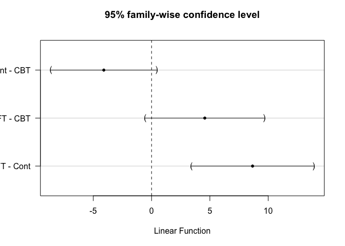
The result suggest each different method is significant in 10% level. Especially, the difference between FT and Cont is 0.1% level.