· Econometrics · 2 min read
One-Way ANOVA
Introduction
Introduction
The hypotheses of one way ANOVA are as follows:
Basically we are going to test the weight differences among the positions in MLB. We chose 5 teams’s 25 active roster data from mlb.com. To perform the analysis, we need to reshape the dataset form the wide to the long form.
library(multcomp) # Multiple Comparisons Package
library(dplyr) #Reshaping data

mlbw = read.csv("mlbw.csv")
id <- rownames(mlbw)
mlbw <- cbind(id=id, mlbw)
mlbl = reshape(data=mlbw, idvar="id",
               varying = c("Pitchers","Infielder","Outfielder"),
               v.name=c("wt"),
               times=c("Pitchers","Infielder","Outfielder"),
               new.row.names = 1:1000,
               direction="long")
mlb<-na.omit(mlbl)
mlb <- mlb %>% rename(pos = time)
mlb$pos = as.factor(mlb$pos)boxplot(wt~pos, data=mlb)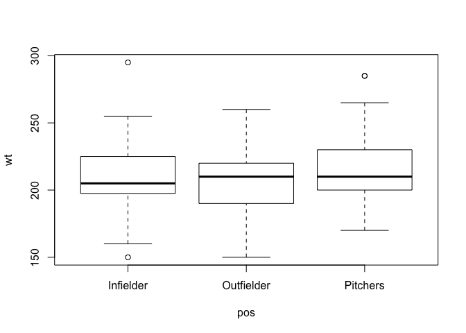
out=lm(wt~pos, data=mlb)
anova(out)
## Analysis of Variance Table
##
## Response: wt
## Df Sum Sq Mean Sq F value Pr(>F)
## pos 2 1734 866.78 1.4528 0.2366
## Residuals 180 107391 596.62Based on the F-value, we cannot reject the null hypothesis, .
par(mfrow=c(2,2))
plot(out)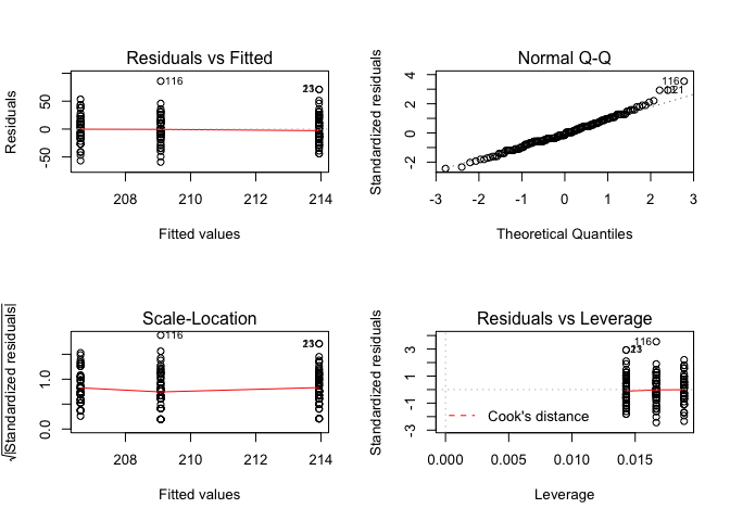
shapiro.test(resid(out))##
## Shapiro-Wilk normality test
##
## data: resid(out)
## W = 0.9864, p-value = 0.07432dunnett = glht(out, linfct= mcp(pos = "Dunnett"))
tukey = glht(out, linfct= mcp(pos = "Tukey"))
summary(dunnett)##
## Simultaneous Tests for General Linear Hypotheses
##
## Multiple Comparisons of Means: Dunnett Contrasts
##
##
## Fit: lm(formula = wt ~ pos, data = mlb)
##
## Linear Hypotheses:
## Estimate Std. Error t value Pr(>|t|)
## Outfielder - Infielder == 0 -2.461 4.604 -0.534 0.814
## Pitchers - Infielder == 0 4.860 4.297 1.131 0.421
## (Adjusted p values reported -- single-step method)Especially, in the case that we can reject the null hypothesis, multiple comparisons are necessary to verify which combination is more significant. There are two famous methods, which are Dunnett and Tukey.
summary(tukey)##
## Simultaneous Tests for General Linear Hypotheses
##
## Multiple Comparisons of Means: Tukey Contrasts
##
##
## Fit: lm(formula = wt ~ pos, data = mlb)
##
## Linear Hypotheses:
## Estimate Std. Error t value Pr(>|t|)
## Outfielder - Infielder == 0 -2.461 4.604 -0.534 0.854
## Pitchers - Infielder == 0 4.860 4.297 1.131 0.496
## Pitchers - Outfielder == 0 7.320 4.447 1.646 0.229
## (Adjusted p values reported -- single-step method)par(mfrow=c(2,1))
plot(dunnett)
plot(tukey)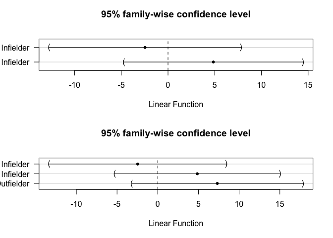
Share: