· Econometrics · 3 min read
Multiple Regression
Analysis and Interpretation
Analysis and Interpretation
Pair Plot to see the correlations among variables
pairs(attitude)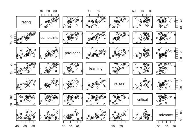
Find the best model
out=lm(rating~., data=attitude)
out2=lm(rating~complaints+learning+advance, data=attitude)
out3=lm(rating~complaints+learning, data=attitude)
anova(out3, out2, out)
## Analysis of Variance Table
##
## Model 1: rating ~ complaints + learning
## Model 2: rating ~ complaints + learning + advance
## Model 3: rating ~ complaints + privileges + learning + raises + critical +
## advance
## Res.Df RSS Df Sum of Sq F Pr(>F)
## 1 27 1254.7
## 2 26 1179.1 1 75.540 1.5121 0.2312
## 3 23 1149.0 3 30.109 0.2009 0.8947Attitude is the data from RStudio. We can get some valuable example to find out the best model by following the step. Using ANOVA, anova(small model, large model), we can compare each model through the F-stat.
summary(out3)##
## Call:
## lm(formula = rating ~ complaints + learning, data = attitude)
##
## Residuals:
## Min 1Q Median 3Q Max
## -11.5568 -5.7331 0.6701 6.5341 10.3610
##
## Coefficients:
## Estimate Std. Error t value Pr(>|t|)
## (Intercept) 9.8709 7.0612 1.398 0.174
## complaints 0.6435 0.1185 5.432 9.57e-06 ***
## learning 0.2112 0.1344 1.571 0.128
## ---
## Signif. codes: 0 '***' 0.001 '**' 0.01 '*' 0.05 '.' 0.1 ' ' 1
##
## Residual standard error: 6.817 on 27 degrees of freedom
## Multiple R-squared: 0.708, Adjusted R-squared: 0.6864
## F-statistic: 32.74 on 2 and 27 DF, p-value: 6.058e-08In this example, the regression model 3, (rating=complaints+learning) is the best among three models.
Another example
We can get the birth weight data from MASS library. To verify which model is better, we are going to run anova() function as before.
library(MASS)
out=lm(bwt~age+lwt+factor(race)+smoke+ptl+ht+ui, data=birthwt)
out2=lm(bwt~lwt+factor(race)+smoke+ht+ui, data=birthwt)

anova(out2, out)
## Analysis of Variance Table
##
## Model 1: bwt ~ lwt + factor(race) + smoke + ht + ui
## Model 2: bwt ~ age + lwt + factor(race) + smoke + ptl + ht + ui
## Res.Df RSS Df Sum of Sq F Pr(>F)
## 1 182 75937505
## 2 180 75741025 2 196480 0.2335 0.792If we remove two variables, ptl and age then the difference in the significance of the model improves a lot.
anova(out2)
summary(out2)
## Analysis of Variance Table
##
## Response: bwt
Df Sum Sq Mean Sq F value Pr(>F)
## lwt 1 3448639 3448639 8.2654 0.0045226 **
## factor(race) 2 5076610 2538305 6.0836 0.0027701 **
## smoke 1 6281818 6281818 15.0557 0.0001458 ***
## ht 1 2871867 2871867 6.8830 0.0094402 **
## ui 1 6353218 6353218 15.2268 0.0001341 ***
## Residuals 182 75937505 417239
## ---
## Signif. codes: 0 ‘***’ 0.001 ‘**’ 0.01 ‘*’ 0.05 ‘.’ 0.1 ‘ ’ 1
## Call:
## lm(formula = bwt ~ lwt + factor(race) + smoke + ht + ui, data = birthwt)
##
## Residuals:
## Min 1Q Median 3Q Max
## -1842.14 -433.19 67.09 459.21 1631.03
##
## Coefficients:
## Estimate Std. Error t value Pr(>|t|)
## (Intercept) 2837.264 243.676 11.644 < 2e-16 ***
## lwt 4.242 1.675 2.532 0.012198 *
## factor(race)2 -475.058 145.603 -3.263 0.001318 **
## factor(race)3 -348.150 112.361 -3.099 0.002254 **
## smoke -356.321 103.444 -3.445 0.000710 ***
## ht -585.193 199.644 -2.931 0.003810 **
## ui -525.524 134.675 -3.902 0.000134 ***
## ---
## Signif. codes: 0 ‘***’ 0.001 ‘**’ 0.01 ‘*’ 0.05 ‘.’ 0.1 ‘ ’ 1
##
## Residual standard error: 645.9 on 182 degrees of freedom
## Multiple R-squared: 0.2404, Adjusted R-squared: 0.2154
## F-statistic: 9.6 on 6 and 182 DF, p-value: 3.601e-09Share: