· International Trade · 3 min read
Nonlinear Regression
Pharmacokinetics
Pharmacokinetics
One of the most important study that applies the nonlinear regression is Pharmacokinetics. It is the study about the absorption, distribution, digestion, and discharge of the drugs.
One Compartment Model
The basic model is as follows:
When you take a drug, the blood concentration has the maximum value as, and then exponentially decreases as time, t, goes. The elimination rate is K.
library("investr")
onecomp=read.csv("data/one_comp.csv")
one=nls(conc~C0*exp(-K*time),start=list(C0=41.3,K=0.64),data=onecomp)
summary(one)
##
## Formula: conc ~ C0 * exp(-K * time)
##
## Parameters:
## Estimate Std. Error t value Pr(>|t|)
## C0 41.76511 1.20688 34.61 4.36e-09 ***
## K 0.64500 0.03236 19.93 2.00e-07 ***
## ---
## Signif. codes: 0 '***' 0.001 '**' 0.01 '*' 0.05 '.' 0.1 ' ' 1
##
## Residual standard error: 1.094 on 7 degrees of freedom
##
## Number of iterations to convergence: 2
## Achieved convergence tolerance: 2.826e-07plotFit(one)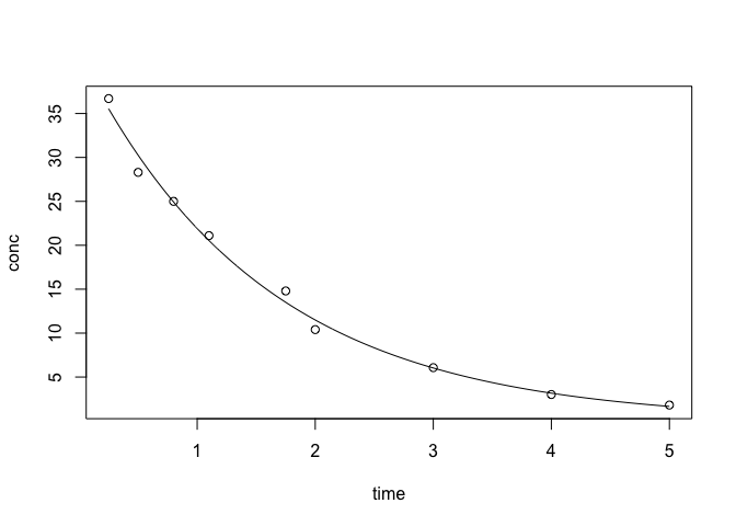
Two Compartment Model
This model is adding one more term in addition to the previous model.
twocomp=read.csv("data/two_comp.csv")
two=nls(conc~SSbiexp(time, A1, lrc1, A2, lrc2), data=twocomp)
summary(two)
##
## Formula: conc ~ SSbiexp(time, A1, lrc1, A2, lrc2)
##
## Parameters:
## Estimate Std. Error t value Pr(>|t|)
## A1 2.0293 0.1099 18.464 3.39e-07 ***
## lrc1 0.5794 0.1247 4.648 0.00235 **
## A2 0.1915 0.1106 1.731 0.12698
## lrc2 -1.7878 0.7871 -2.271 0.05737 .
## ---
## Signif. codes: 0 '***' 0.001 '**' 0.01 '*' 0.05 '.' 0.1 ' ' 1
##
## Residual standard error: 0.04103 on 7 degrees of freedom
##
## Number of iterations to convergence: 0
## Achieved convergence tolerance: 4.225e-06plotFit(two)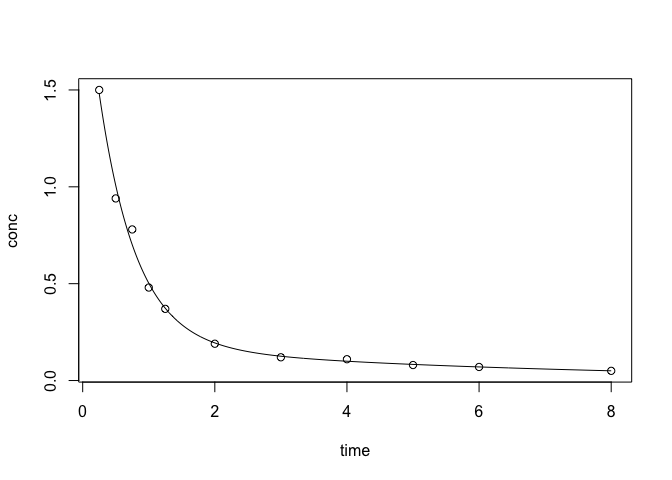
One Compartment Model : Oral Dosage
This model shows the blood concentration when the drug is taken by oral dosage.
oraldose=read.csv("data/oral_dose.csv")
oral=nls(conc~SSfol(Dose=4.4, time, lKe, lKa, lCl), data=oraldose)
summary(oral)
##
## Formula: conc ~ SSfol(Dose = 4.4, time, lKe, lKa, lCl)
##
## Parameters:
## Estimate Std. Error t value Pr(>|t|)
## lKe -2.2861 0.2491 -9.178 1.60e-05 ***
## lKa 0.6641 0.2966 2.239 0.0556 .
## lCl -3.1063 0.1643 -18.907 6.33e-08 ***
## ---
## Signif. codes: 0 '***' 0.001 '**' 0.01 '*' 0.05 '.' 0.1 ' ' 1
##
## Residual standard error: 1.058 on 8 degrees of freedom
##
## Number of iterations to convergence: 7
## Achieved convergence tolerance: 4.668e-06plotFit(oral, xlim=c(0,35))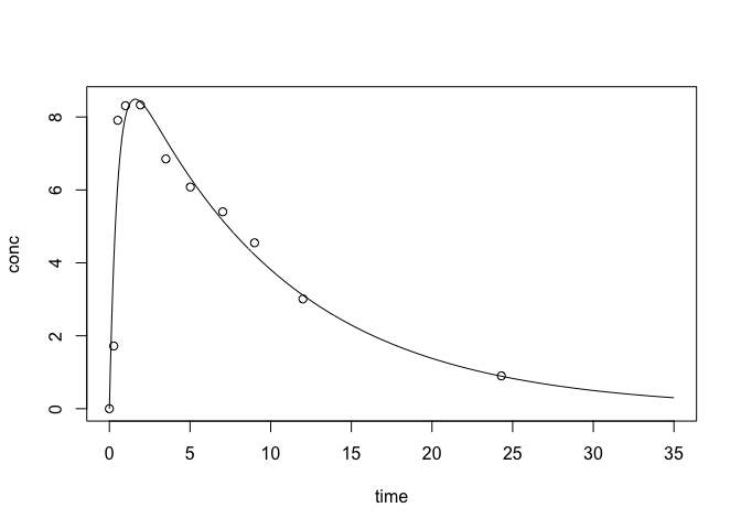
Michaelis-Menten Model
mime=read.csv("data/MM.csv")
mm=nls(rate~SSmicmen(conc,Vm,K), data=mime)
summary(mm)
##
## Formula: rate ~ SSmicmen(conc, Vm, K)
##
## Parameters:
## Estimate Std. Error t value Pr(>|t|)
## Vm 126.033 7.173 17.570 2.18e-06 ***
## K 17.079 2.953 5.784 0.00117 **
## ---
## Signif. codes: 0 '***' 0.001 '**' 0.01 '*' 0.05 '.' 0.1 ' ' 1
##
## Residual standard error: 6.25 on 6 degrees of freedom
##
## Number of iterations to convergence: 0
## Achieved convergence tolerance: 2.522e-06plotFit(mm, ylim=c(0,130), xlim=c(0,400))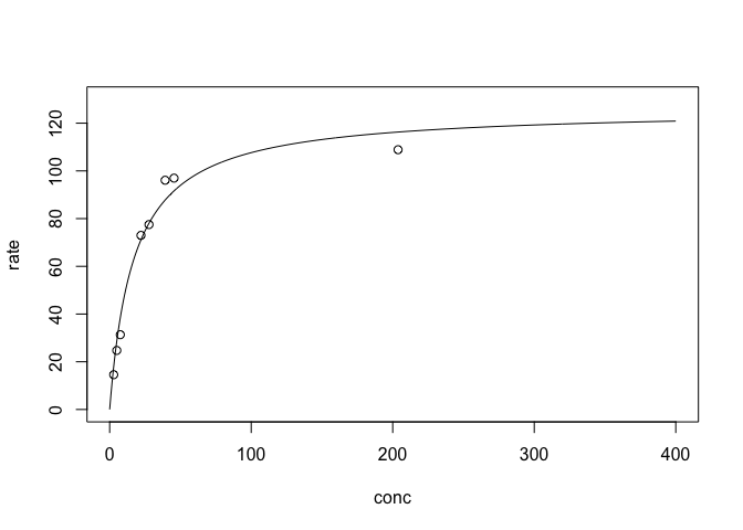
Share: