· Econometrics · 3 min read
Two-Way ANOVA
Data
Data
This data is SAT scores and GPA for every student who entered the University of Texas at Austin at 2000 and graduated within 6 years. As a two-way ANOVA model, we want to analyze the impact from 2 factor variables as well as the interaction between them.
sat = read.csv("ut2000.csv")
attach(sat)
tapply(SAT.C, list(Gender,School),mean)
## ARCHITECTURE BUSINESS COMMUNICATIONS EDUCATION ENGINEERING FINE ARTS
## F 1338.500 1232.114 1204.792 1105.645 1279.062 1186.133
## M 1359.167 1228.418 1197.099 1096.750 1284.111 1195.062
## LIBERAL ARTS NATURAL SCIENCE NURSING SOCIAL WORK
## F 1183.540 1234.531 1114.231 1168.333
## M 1190.767 1226.107 1119.375 1208.750boxplot(SAT.Q~Gender+School, col="blue", data=sat)
interaction.plot(Gender, School, SAT.Q, col=c("blue","red"))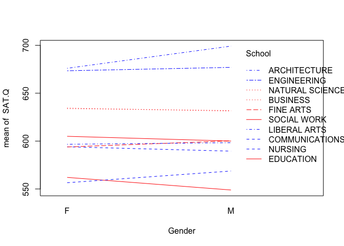
out=lm(SAT.Q~Gender*School,data=sat)
out1=lm(SAT.Q~Gender+School+Gender*School,data=sat)
out2=lm(SAT.Q~Gender+School,data=sat)

anova(out)
## Analysis of Variance Table
##
## Response: SAT.Q
## Df Sum Sq Mean Sq F value Pr(>F)
## Gender 1 1565 1565 0.2592 0.6107
## School 9 4592051 510228 84.5374 <2e-16 ***
## Gender:School 9 21355 2373 0.3931 0.9390
## Residuals 5171 31209727 6036
## ---
## Signif. codes: 0 '***' 0.001 '**' 0.01 '*' 0.05 '.' 0.1 ' ' 1summary(out1)##
## Call:
## lm(formula = SAT.Q ~ Gender + School + Gender * School, data = sat)
##
## Residuals:
## Min 1Q Median 3Q Max
## -311.338 -51.911 1.695 53.301 205.972
##
## Coefficients:
## Estimate Std. Error t value Pr(>|t|)
## (Intercept) 676.000 17.372 38.914 < 2e-16 ***
## GenderM 23.167 28.368 0.817 0.4142
## SchoolBUSINESS -41.534 17.780 -2.336 0.0195 *
## SchoolCOMMUNICATIONS -81.972 18.539 -4.422 1.00e-05 ***
## SchoolEDUCATION -113.903 19.978 -5.701 1.25e-08 ***
## SchoolENGINEERING -2.591 17.858 -0.145 0.8847
## SchoolFINE ARTS -82.133 19.551 -4.201 2.70e-05 ***
## SchoolLIBERAL ARTS -79.301 17.559 -4.516 6.44e-06 ***
## SchoolNATURAL SCIENCE -42.106 17.677 -2.382 0.0173 *
## SchoolNURSING -119.462 23.107 -5.170 2.43e-07 ***
## SchoolSOCIAL WORK -71.000 36.162 -1.963 0.0497 *
## GenderM:SchoolBUSINESS -26.294 28.875 -0.911 0.3625
## GenderM:SchoolCOMMUNICATIONS -27.688 29.731 -0.931 0.3517
## GenderM:SchoolEDUCATION -36.388 31.265 -1.164 0.2445
## GenderM:SchoolENGINEERING -19.608 28.974 -0.677 0.4986
## GenderM:SchoolFINE ARTS -16.786 30.979 -0.542 0.5879
## GenderM:SchoolLIBERAL ARTS -21.561 28.597 -0.754 0.4509
## GenderM:SchoolNATURAL SCIENCE -25.150 28.744 -0.875 0.3816
## GenderM:SchoolNURSING -10.955 37.604 -0.291 0.7708
## GenderM:SchoolSOCIAL WORK -28.167 50.647 -0.556 0.5781
## ---
## Signif. codes: 0 '***' 0.001 '**' 0.01 '*' 0.05 '.' 0.1 ' ' 1
##
## Residual standard error: 77.69 on 5171 degrees of freedom
## Multiple R-squared: 0.1288, Adjusted R-squared: 0.1256
## F-statistic: 40.24 on 19 and 5171 DF, p-value: < 2.2e-16summary(out2)##
## Call:
## lm(formula = SAT.Q ~ Gender + School, data = sat)
##
## Residuals:
## Min 1Q Median 3Q Max
## -312.870 -52.870 2.446 52.546 208.313
##
## Coefficients:
## Estimate Std. Error t value Pr(>|t|)
## (Intercept) 684.72488 13.75012 49.798 < 2e-16 ***
## GenderM -0.09969 2.15720 -0.046 0.963142
## SchoolBUSINESS -51.75496 13.99014 -3.699 0.000218 ***
## SchoolCOMMUNICATIONS -93.03812 14.43002 -6.448 1.24e-10 ***
## SchoolEDUCATION -130.02083 15.19985 -8.554 < 2e-16 ***
## SchoolENGINEERING -9.51022 14.04108 -0.677 0.498237
## SchoolFINE ARTS -87.49363 15.07172 -5.805 6.81e-09 ***
## SchoolLIBERAL ARTS -87.17084 13.84738 -6.295 3.32e-10 ***
## SchoolNATURAL SCIENCE -51.76859 13.92267 -3.718 0.000203 ***
## SchoolNURSING -123.49643 18.21986 -6.778 1.35e-11 ***
## SchoolSOCIAL WORK -82.52506 24.88465 -3.316 0.000918 ***
## ---
## Signif. codes: 0 '***' 0.001 '**' 0.01 '*' 0.05 '.' 0.1 ' ' 1
##
## Residual standard error: 77.65 on 5180 degrees of freedom
## Multiple R-squared: 0.1282, Adjusted R-squared: 0.1265
## F-statistic: 76.19 on 10 and 5180 DF, p-value: < 2.2e-16par(mfrow=c(2,2))
plot(out)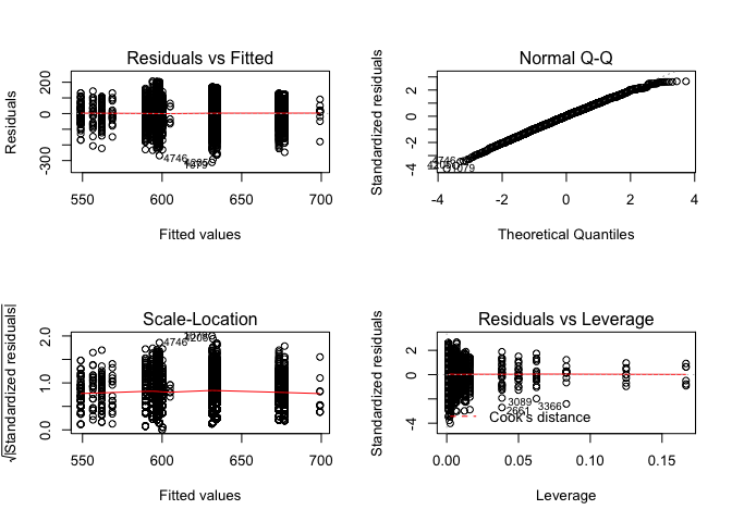
Share: